A forecast that says the Chiefs have a 70% chance to win is making a claim you can check. The trouble is that one game can’t tell you whether 70% was right. If the Chiefs win, the forecast looks good. If they lose, it may still have been a fair number, since 70% means losing 3 times out of 10.
So forecasts are graded over many games, with scores built for probabilities. This post covers the three that matter most: log loss, calibration, and the Brier score. These are the same measures the bayesRatings scorecard uses.
Why win percentage isn’t enough
The simplest grade is how often the favorite won. It’s useful, but it throws away the number itself. Take two forecasters who pick the same team in every game. One says 55%, the other 95%. Their win percentage is identical. But if the favorite wins only 55% of the time, the first told you the truth and the second was badly overconfident.
A good grade has to reward the right number, not just the right side.
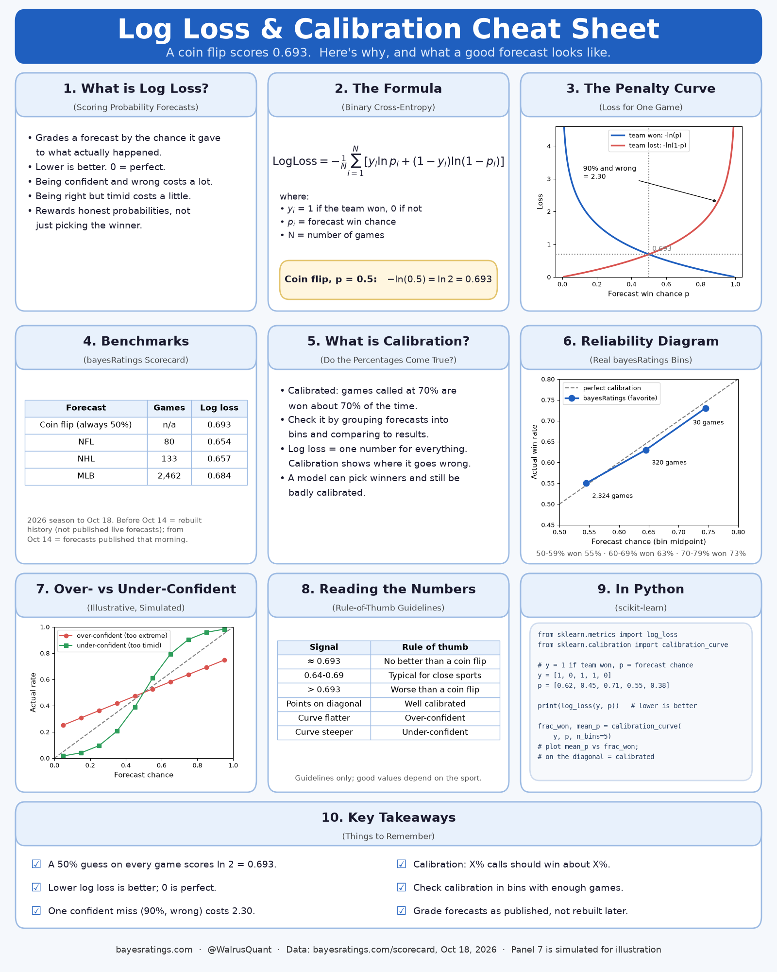
Log loss
Log loss scores each game on the chance you gave the team that actually won. Take the natural log of that chance and flip the sign:
Log loss for one game = −ln(chance you gave the winner)
Averaged over N games, with p as your chance for a team and y = 1 if that team won, 0 if not:
Log loss = −(1/N) Σ [ y·ln(p) + (1 − y)·ln(1 − p) ]
Lower is better. Some examples:
- You say 70% and the team wins: −ln(0.70) = 0.36
- You say 70% and the team loses: −ln(0.30) = 1.20
- You say 90% and the team wins: −ln(0.90) = 0.11
- You say 90% and the team loses: −ln(0.10) = 2.30
That last line is the key feature. Being confident and right saves you a little. Being confident and wrong costs you a lot. Say 99% and lose, and that one game costs 4.61. There’s no upper limit.
The baseline is 0.693. If you call every game 50/50, every game costs −ln(0.5) = ln 2 = 0.693, no matter who wins. A forecast has to score below 0.693 to tell you more than a coin flip.
As of Oct 18, 2026, the bayesRatings scorecard shows:
| League | Games | Favorite won | Log loss | Brier score |
|---|---|---|---|---|
| NFL | 80 | 57% | 0.654 | 0.232 |
| NHL | 133 | 61% | 0.657 | 0.233 |
| MLB | 2,462 | 56% | 0.684 | 0.246 |
| Coin flip | n/a | n/a | 0.693 | 0.25 |
One way to read these: a log loss of 0.654 means the forecast gave the winning team about a 52% chance on average (a geometric average: e^−0.654 ≈ 0.52). That sounds small, but sports are close. MLB sits near 0.693 because baseball games are close to toss-ups, and even a good forecast rarely moves far from 50%.
Calibration
Calibration asks a direct question: when you say 60%, does it happen about 60% of the time? If you give 100 teams a 60% chance, about 60 of them should win. If only 50 do, you’re overconfident. If 70 do, you’re underconfident.
To check it, group forecasts into bins and compare each bin with what happened. Here is the scorecard’s version for all graded games as of Oct 18, 2026:
| Chance given to the favorite | Games | Favorite won |
|---|---|---|
| 50-59% | 2,324 | 55% |
| 60-69% | 320 | 63% |
| 70-79% | 30 | 73% |
All three bins land inside their ranges. Favorites given 50 to 59% won 55% of the time, favorites given 60 to 69% won 63%, and favorites given 70 to 79% won 73%. That’s what a calibrated forecast looks like. The 70 to 79% bin is small (only 30 games), so read it as a rough check. The 50 to 59% bin holds most of the games because most are MLB, where few games are lopsided.
Calibration alone isn’t enough, though. A forecaster who says 50% for every game is perfectly calibrated if home and away teams each win half the time, yet tells you nothing. You need both: percentages that come true and percentages that move away from 50% when the games call for it. Log loss rewards both at once. That’s why the scorecard reports log loss and the calibration table together.
Brier score
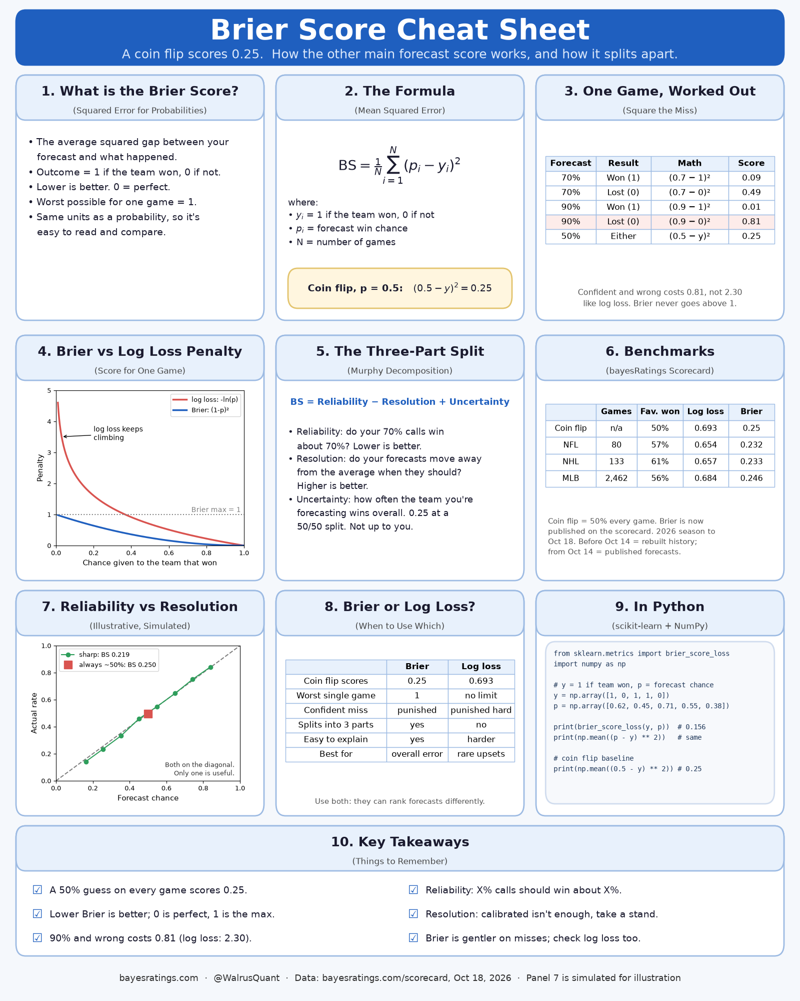
The Brier score is the other main way to grade a probability forecast. For each game, take the chance you gave, subtract what happened (1 if the team won, 0 if not), and square it. Then average over every game:
Brier score = (1/N) Σ (p − y)²
Lower is better, 0 is perfect, and one game can never cost more than 1. With the same examples as above:
- You say 70% and the team wins: (0.7 − 1)² = 0.09
- You say 70% and the team loses: (0.7 − 0)² = 0.49
- You say 90% and the team wins: (0.9 − 1)² = 0.01
- You say 90% and the team loses: (0.9 − 0)² = 0.81
The baseline is 0.25. Calling every game 50/50 always scores (0.5 − 1)² = (0.5 − 0)² = 0.25.
The useful part of the Brier score is that it splits into three pieces:
- Reliability. Do your 70% calls actually win about 70% of the time? This is calibration as a number. Lower is better.
- Resolution. Do your forecasts move away from the overall average when they should? A forecaster who says 50% every game scores zero here. Higher is better.
- Uncertainty. How often the team you’re forecasting wins overall. If the base rate is r, uncertainty is r × (1 − r). At a 50/50 split it’s 0.25. If the favorite wins 56% of the time, it’s 0.56 × 0.44 = 0.246. This piece isn’t up to you.
Brier score = reliability − resolution + uncertainty
The always-50% forecaster shows how this works. If teams win half the time, reliability is 0, resolution is 0, and uncertainty is 0.25, so the Brier score is 0.25. To get below that, a forecast has to earn resolution without giving it back in reliability. (The three parts add up exactly when forecasts are grouped into bins, like 60 to 69%.)
On the scorecard this season, NFL scores 0.232, NHL 0.233 and MLB 0.246, all below the 0.25 coin flip. MLB sits closest to 0.25 because baseball games are near toss-ups.
Log loss vs. Brier score
Both scores reward honest, confident forecasts, and both have a best possible score of 0. The difference is how hard they punish a confident miss.
| Log loss | Brier score | |
|---|---|---|
| Coin flip (50% every game) | 0.693 | 0.25 |
| 70% and wrong | 1.20 | 0.49 |
| 90% and wrong | 2.30 | 0.81 |
| 99% and wrong | 4.61 | 0.98 |
| Worst single game | No limit | 1 |
| Splits into three parts | No | Yes |
| Most sensitive to | Upsets you were sure wouldn’t happen | Overall error |
Going from a 70% miss to a 90% miss almost doubles the log loss penalty (1.20 to 2.30). The Brier penalty grows much less (0.49 to 0.81). So log loss cares most about games where you were sure and wrong. Brier measures overall error and is easier to break apart.
They can also rank forecasts differently. A forecaster who is usually sharp but sometimes says 95% on a game that goes the other way can look fine on Brier and poor on log loss. If you care about not being blindsided, log loss is the stricter test. It’s worth checking both.
How bayesRatings is graded
Every bayesRatings forecast is graded once the game ends, and the results are on the scorecard. It shows how often the favorite won, the log loss and Brier score for each league, and the calibration table above. The scorecard also grades the Kalshi pre-game market price the same way, on the same games, as a reference point.
The current model went live on Oct 14, 2026. From that date on, each forecast is the one published that morning. Games before Oct 14 were forecast after the fact with the current model, using only games played before each day. The NBA season starts Oct 20.
The methodology page explains how the ratings and forecasts are built, and what the model does and doesn’t use yet.
Takeaways
- Win percentage tells you whether the pick was right, not whether the number was right.
- Log loss: lower is better, a coin flip scores 0.693, and a 90% miss costs 2.30.
- Calibration: when a forecast says 60%, it should happen about 60% of the time.
- Brier score: lower is better, a coin flip scores 0.25, and no game costs more than 1.
- Brier = reliability − resolution + uncertainty. Calibrated isn’t enough; a forecast also has to move off 50% when it should.
- Check both scores. Log loss is the stricter test on confident misses.